EDA란?
EDA(Exploratory Data Analysis, 탐색적 데이터 분석)는 수집한 데이터를 그래프와 통계적 방법으로 직관적으로 이해하고 숨겨진 패턴이나 오류를 찾는 과정을 의미한다.
EDA는 데이터를 모델에 넣기 전에 아래 내용을 확인하는 과정이다.
- 데이터가 어떤 구조인지
- 결측치나 이상치가 있는지
- 결과값(타겟값)와 어떤 변수들이 관련 있어 보이는지
- 전처리 과정에서 무엇을 바꿔야 하는지
- 모델 학습에 쓰면 안 되는 정보 누수(leakage) 변수가 있는지
0. 데이터셋 준비하기
여기서 CSV 데이터셋을 다운로드한다. 주요 컬럼을 정리하자면 다음과 같다.
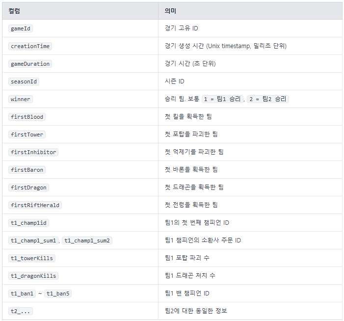
문제 정의: 우리의 목표는 랭크게임 데이터를 기반으로 승리에 영향을 미치는 요인을 분석하는 것이다.
1. 라이브러리 불러오기 및 데이터 읽기
import numpy as np
import pandas as pd
import matplotlib.pyplot as plt
import seaborn as sns

# 그래프 스타일 설정
sns.set_theme(style="whitegrid")

# CSV 읽기
df = pd.read_csv("dataset/games.csv")

# 한글 폰트 설정
plt.rcParams["font.family"] = "Malgun Gothic"
plt.rcParams["axes.unicode_minus"] = False
2. 데이터 구조 확인하기
EDA의 시작은 "데이터가 어떻게 생겼는가?"를 확인하는 것이다.
# 기본 데이터 조회
print(df.head()) # 상위 5개 행 확인
print(df.tail()) # 하위 5개 행 확인
print(df.shape)  # 데이터가 몇 개의 행과 열로 이루어져 있는지 확인
print(df.columns.tolist()) # 컬럼 목록 확인
print(df.info())  # 컬럼별 데이터 타입 및 결측치 여부 확인
print(df.describe()) # 기초 통계량 확인# df.head()
gameId creationTime gameDuration seasonId winner ... t2_ban1 t2_ban2 t2_ban3 t2_ban4 t2_ban5
0 3326086514 1504279457970 1949 9 1 ... 114 67 43 16 51
1 3229566029 1497848803862 1851 9 1 ... 11 67 238 51 420
2 3327363504 1504360103310 1493 9 1 ... 157 238 121 57 28
3 3326856598 1504348503996 1758 9 1 ... 164 18 141 40 51
4 3330080762 1504554410899 2094 9 1 ... 86 11 201 122 18
[5 rows x 61 columns]
#--------------------
# df.tail()
gameId creationTime gameDuration seasonId winner ... t2_ban1 t2_ban2 t2_ban3 t2_ban4 t2_ban5
51485 3308904636 1503076540231 1944 9 2 ... 55 -1 90 238 157
51486 3215685759 1496957179355 3304 9 2 ... 157 55 119 154 105
51487 3322765040 1504029863961 2156 9 2 ... 113 122 53 11 157
51488 3256675373 1499562036246 1475 9 2 ... 154 39 51 90 114
51489 3317333020 1503612754059 1445 9 1 ... 11 157 141 31 18
[5 rows x 61 columns]
#--------------------
# df.shape
(51490, 61)
#--------------------
# df.columns.tolist()
['gameId', 'creationTime', 'gameDuration', 'seasonId', 'winner', 'firstBlood', 'firstTower', 'firstInhibitor', 'firstBaron', 'firstDragon', 'firstRiftHerald', 't1_champ1id', 't1_champ1_sum1', 't1_champ1_sum2', 't1_champ2id', 't1_champ2_sum1', 't1_champ2_sum2', 't1_champ3id', 't1_champ3_sum1', 't1_champ3_sum2', 't1_champ4id', 't1_champ4_sum1', 't1_champ4_sum2', 't1_champ5id', 't1_champ5_sum1', 't1_champ5_sum2', 't1_towerKills', 't1_inhibitorKills', 't1_baronKills', 't1_dragonKills', 't1_riftHeraldKills', 't1_ban1', 't1_ban2', 't1_ban3', 't1_ban4', 't1_ban5', 't2_champ1id', 't2_champ1_sum1', 't2_champ1_sum2', 't2_champ2id', 't2_champ2_sum1', 't2_champ2_sum2', 't2_champ3id', 't2_champ3_sum1', 't2_champ3_sum2', 't2_champ4id', 't2_champ4_sum1', 't2_champ4_sum2', 't2_champ5id', 't2_champ5_sum1', 't2_champ5_sum2', 't2_towerKills', 't2_inhibitorKills', 't2_baronKills', 't2_dragonKills', 't2_riftHeraldKills', 't2_ban1', 't2_ban2', 't2_ban3', 't2_ban4', 't2_ban5']
#--------------------
# df.info()
<class 'pandas.DataFrame'>
RangeIndex: 51490 entries, 0 to 51489
Data columns (total 61 columns):
# Column Non-Null Count Dtype
--- ------ -------------- -----
0 gameId 51490 non-null int64
1 creationTime 51490 non-null int64
2 gameDuration 51490 non-null int64
3 seasonId 51490 non-null int64
4 winner 51490 non-null int64
5 firstBlood 51490 non-null int64
6 firstTower 51490 non-null int64
7 firstInhibitor 51490 non-null int64
8 firstBaron 51490 non-null int64
9 firstDragon 51490 non-null int64
10 firstRiftHerald 51490 non-null int64
11 t1_champ1id 51490 non-null int64
12 t1_champ1_sum1 51490 non-null int64
13 t1_champ1_sum2 51490 non-null int64
14 t1_champ2id 51490 non-null int64
15 t1_champ2_sum1 51490 non-null int64
16 t1_champ2_sum2 51490 non-null int64
17 t1_champ3id 51490 non-null int64
18 t1_champ3_sum1 51490 non-null int64
19 t1_champ3_sum2 51490 non-null int64
20 t1_champ4id 51490 non-null int64
21 t1_champ4_sum1 51490 non-null int64
22 t1_champ4_sum2 51490 non-null int64
23 t1_champ5id 51490 non-null int64
24 t1_champ5_sum1 51490 non-null int64
25 t1_champ5_sum2 51490 non-null int64
26 t1_towerKills 51490 non-null int64
27 t1_inhibitorKills 51490 non-null int64
28 t1_baronKills 51490 non-null int64
29 t1_dragonKills 51490 non-null int64
30 t1_riftHeraldKills 51490 non-null int64
31 t1_ban1 51490 non-null int64
32 t1_ban2 51490 non-null int64
33 t1_ban3 51490 non-null int64
34 t1_ban4 51490 non-null int64
35 t1_ban5 51490 non-null int64
36 t2_champ1id 51490 non-null int64
37 t2_champ1_sum1 51490 non-null int64
38 t2_champ1_sum2 51490 non-null int64
39 t2_champ2id 51490 non-null int64
40 t2_champ2_sum1 51490 non-null int64
41 t2_champ2_sum2 51490 non-null int64
42 t2_champ3id 51490 non-null int64
43 t2_champ3_sum1 51490 non-null int64
44 t2_champ3_sum2 51490 non-null int64
45 t2_champ4id 51490 non-null int64
46 t2_champ4_sum1 51490 non-null int64
47 t2_champ4_sum2 51490 non-null int64
48 t2_champ5id 51490 non-null int64
49 t2_champ5_sum1 51490 non-null int64
50 t2_champ5_sum2 51490 non-null int64
51 t2_towerKills 51490 non-null int64
52 t2_inhibitorKills 51490 non-null int64
53 t2_baronKills 51490 non-null int64
54 t2_dragonKills 51490 non-null int64
55 t2_riftHeraldKills 51490 non-null int64
56 t2_ban1 51490 non-null int64
57 t2_ban2 51490 non-null int64
58 t2_ban3 51490 non-null int64
59 t2_ban4 51490 non-null int64
60 t2_ban5 51490 non-null int64
dtypes: int64(61)
memory usage: 24.0 MB
None
#--------------------
# df.describe()
gameId creationTime gameDuration seasonId ... t2_ban2 t2_ban3 t2_ban4 t2_ban5
count 5.149000e+04 5.149000e+04 51490.000000 51490.0 ... 51490.000000 51490.000000 51490.000000 51490.000000
mean 3.306223e+09 1.502926e+12 1832.362808 9.0 ... 107.910216 108.690581 108.626044 108.066576
std 2.946096e+07 1.978026e+09 512.017696 0.0 ... 102.870710 102.592145 103.346952 102.756149
min 3.214824e+09 1.496892e+12 190.000000 9.0 ... -1.000000 -1.000000 -1.000000 -1.000000
25% 3.292218e+09 1.502021e+12 1531.000000 9.0 ... 37.000000 38.000000 38.000000 38.000000
50% 3.320021e+09 1.503844e+12 1833.000000 9.0 ... 90.000000 90.000000 90.000000 90.000000
75% 3.327099e+09 1.504352e+12 2148.000000 9.0 ... 141.000000 141.000000 141.000000 141.000000
max 3.331833e+09 1.504707e+12 4728.000000 9.0 ... 516.000000 516.000000 516.000000 516.000000
[8 rows x 61 columns]3-1. 결측치 확인
# 컬럼별 결측치 확인
print(df.isnull().sum())

# 결측치가 있는 컬럼만 확인
missing = df.isnull().sum()
print(missing[missing > 0].sort_values(ascending=False))

# 결측치 비율 확인
missing_ratio = df.isnull().mean() * 100
print(missing_ratio[missing_ratio > 0].sort_values(ascending=False))

'''
gameId          0
creationTime    0
gameDuration    0
seasonId        0
winner          0
               ..
t2_ban1         0
t2_ban2         0
t2_ban3         0
t2_ban4         0
t2_ban5         0
Length: 61, dtype: int64
--------------------
Series([], dtype: int64)
--------------------
Series([], dtype: float64)
'''
현재 사용중인 데이터셋에서는 결측치가 없지만, 실제로는 결측치가 없는 경우가 드물 것이다.
3-2. 결측치 처리
- 숫자형 데이터: 중앙값으로 채우기
df["gameDuration"] = df["gameDuration"].fillna(df["gameDuration"].median())- 범주형 데이터: 최빈값 또는 별도 값으로 채우기
df["t1_ban1"] = df["t1_ban1"].fillna(-1)4. 중복 데이터 확인
동일한 데이터가 여러 번 들어가 있다면 모델 학습 결과가 왜곡될 수 있다.
# 중복 데이터 확인
print(f"중복 제거 전: {df["gameId"].duplicated().sum()}")
df = df.drop_duplicates(subset="gameId")
print(f"중복 제거 후: {df["gameId"].duplicated().sum()}")

'''
중복 제거 전: 437
중복 제거 후: 0
'''
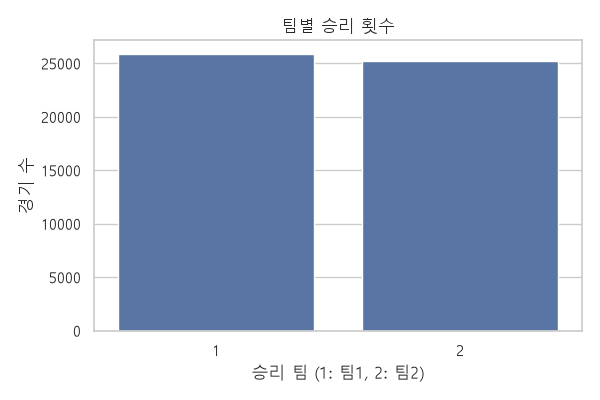
5-1. 타겟 변수 winner 분석
# winner 분석
print(df["winner"].value_counts())
print(df["winner"].value_counts(normalize=True) * 100)
plt.figure(figsize=(6, 4))
sns.countplot(data=df, x="winner")
plt.title("팀별 승리 횟수")
plt.xlabel("승리 팀 (1: 팀1, 2: 팀2)")
plt.ylabel("경기 수")
plt.tight_layout() # 라벨 짤림 방지
plt.show()

'''
winner
1    25857
2    25196
Name: count, dtype: int64
winner
1    50.647366
2    49.352634
Name: proportion, dtype: float64
'''
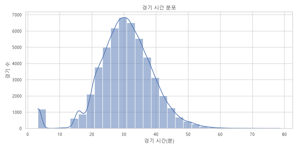
5-2. 경기 시간 분석
# 경기 시간 분석
df["gameDuration_min"] = df["gameDuration"] / 60 # 초 → 분 단위 변환

plt.figure(figsize=(10, 5))
sns.histplot(
    data=df,
    x="gameDuration_min",
    bins=30,
    kde=True
)
plt.title("경기 시간 분포")
plt.xlabel("경기 시간(분)")
plt.ylabel("경기 수")
plt.tight_layout()
plt.show() # Fig 1

plt.figure(figsize=(8, 5))
sns.boxplot(
    data=df,
    x="winner",
    y="gameDuration_min"
)
plt.title("승리 팀에 따른 경기 시간 분포")
plt.xlabel("승리 팀")
plt.ylabel("경기 시간(분)")
plt.show() # Fig 2| Fig 1 | Fig 2 |
 |
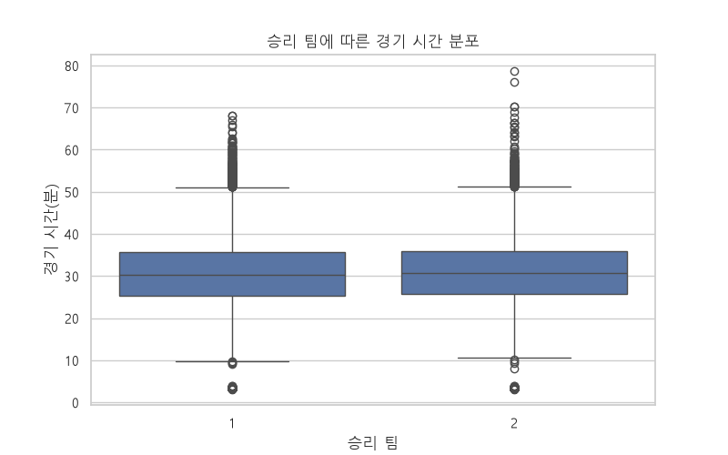 |
⚠️ 경기 시간은 경기 종료 후에 알 수 있는 값이므로, 게임 시작 전에 승패를 예측할 수 있는 모델을 만들고 싶다면 gameDuration은 사용할 수 없다.
5-3. 오브젝트와 승리의 관계 살펴보기
# 오브젝트와 승리의 관계 분석
first_columns = [
    "firstBlood",
    "firstTower",
    "firstInhibitor",
    "firstBaron",
    "firstDragon",
    "firstRiftHerald"
]

fig, axes = plt.subplots(2, 3, figsize=(15, 9))
axes = axes.flatten()

for i, col in enumerate(first_columns):
    sns.countplot(data=df, x=col, hue="winner", ax=axes[i])
    axes[i].set_title(f"{col}와 승리 팀의 관계")
    axes[i].set_xlabel(col)
    axes[i].set_ylabel("경기 수")

plt.tight_layout()
plt.show()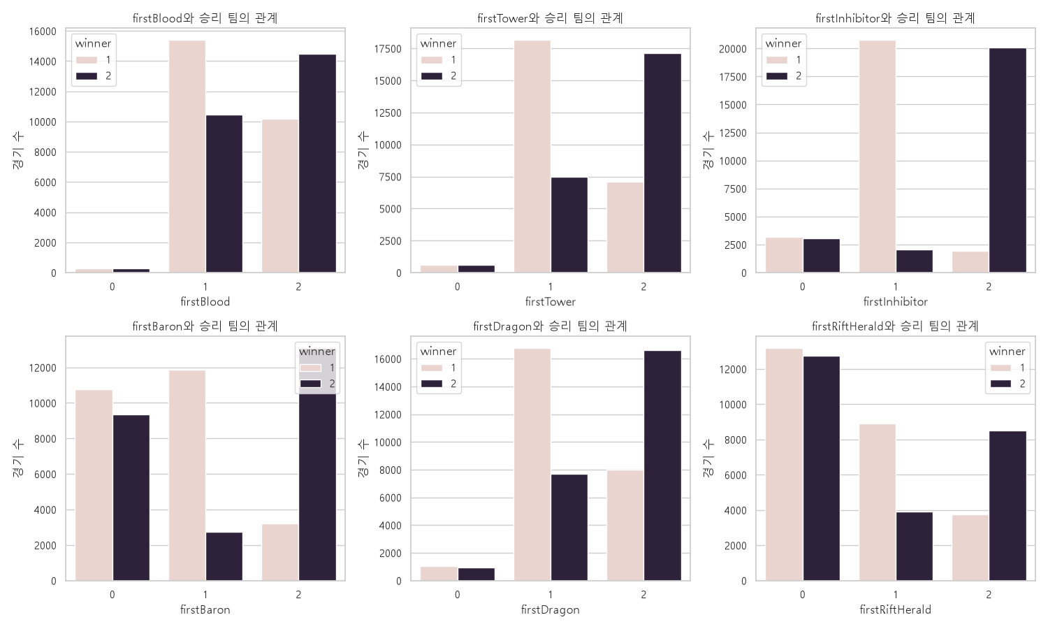
firstTower=1일 때 winner=1이 많은 것을 보고 "첫 포탑을 가져간 팀이 경기에서 이기는 비율이 높다"고 해석할 수 있다. 하지만 EDA에서는 관계와 패턴만 파악해야지, 인과관계로 해석하 면 안 된다.
5-4. 팀별 오브젝트 처치 수 비교
# 팀별 오브젝트 처치 수 비교
objectives = [
    "towerKills",
    "inhibitorKills",
    "baronKills",
    "dragonKills",
    "riftHeraldKills",
]

df_melted = pd.melt(
    df,
    value_vars=[f"t1_{obj}" for obj in objectives]
    + [f"t2_{obj}" for obj in objectives],
    var_name="Column",
    value_name="Kills",
)

df_melted["Team"] = df_melted["Column"].apply(
    lambda x: "Team 1" if x.startswith("t1_") else "Team 2"
)
df_melted["Objective"] = df_melted["Column"].apply(
    lambda x: x.replace("t1_", "").replace("t2_", "").replace("Kills", "")
)

plt.figure(figsize=(12, 6))
sns.barplot(
    data=df_melted, x="Objective", y="Kills", hue="Team", errorbar=None
)

plt.title("팀별 주요 오브젝트 평균 처치 수 비교", fontsize=14)
plt.xlabel("오브젝트 종류", fontsize=12)
plt.ylabel("평균 처치 수", fontsize=12)
plt.grid(axis="y", linestyle="--", alpha=0.7)
plt.tight_layout()
plt.show()
6. 팀 간 차이 변수 만들기
원래 데이터에는 팀1과 팀2의 정보가 따로 있는데, 모델링이나 분석에서는 두 팀의 차이값이 더 유용할 수 있다.
# 팀 간 차이 변수 만들기
df["tower_diff"] = df["t1_towerKills"] - df["t2_towerKills"]
df["inhibitor_diff"] = df["t1_inhibitorKills"] - df["t2_inhibitorKills"]
df["baron_diff"] = df["t1_baronKills"] - df["t2_baronKills"]
df["dragon_diff"] = df["t1_dragonKills"] - df["t2_dragonKills"]
df["riftHerald_diff"] = df["t1_riftHeraldKills"] - df["t2_riftHeraldKills"]

plt.figure(figsize=(8, 5))
sns.boxplot(
    data=df,
    x="winner",
    y="tower_diff"
)
plt.axhline(0, color="black", linestyle="--")
plt.title("승리 팀에 따른 포탑 파괴 수 차이")
plt.xlabel("승리 팀")
plt.ylabel("팀1 포탑 수 - 팀2 포탑 수")
plt.show()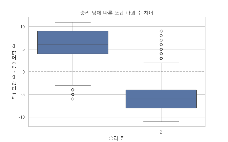
7. 상관관계 확인
numeric_cols = [
    "gameDuration",
    "t1_towerKills", "t2_towerKills",
    "t1_inhibitorKills", "t2_inhibitorKills",
    "t1_baronKills", "t2_baronKills",
    "t1_dragonKills", "t2_dragonKills",
    "t1_riftHeraldKills", "t2_riftHeraldKills"
]

corr = df[numeric_cols].corr()
plt.figure(figsize=(12, 8))
sns.heatmap(corr, annot=True, cmap="coolwarm", fmt=".2f")
plt.title("상관관계 히트맵")
plt.tight_layout()
plt.show()
- 상관관계가 높다고 해서 인과관계인 것은 아니다.
- ID값은 숫자이지만, 크기에 의미가 없기 때문에 상관관계 해석에 적합하지 않다.
8. creationTime 전처리
데이터 전처리는 수집한 raw 데이터를 인공지능 모델 학습이나 데이터 분석에 적합한 깨끗하고 유용한 형태로 가공하는 과정
이다. 불순물을 제거하는 정제 작업부터 형태를 바꾸는 변환 작업까지 포함하며, 최종 결과의 품질을 좌우하는 필수적인 단계이다.
creationTime은 1504279457970와 같이 ms 단위의 큰 숫자값으로 저장되어 있는데, 이를 사람이 읽을 수 있는 값으로 변환할 수 있다.
# creationTime 전처리
df["creationTime"] = pd.to_datetime(
    df["creationTime"],
    unit="ms"
)
print(df[["creationTime"]].head())
'''
             creationTime
0 2017-09-01 15:24:17.970
1 2017-06-19 05:06:43.862
2 2017-09-02 13:48:23.310
3 2017-09-02 10:35:03.996
4 2017-09-04 19:46:50.899
'''

# 연도, 월, 요일 등 새 특성을 만들수도 있음
df["year"] = df["creationTime"].dt.year
df["month"] = df["creationTime"].dt.month
df["dayofweek"] = df["creationTime"].dt.dayofweek
다만 날짜 자체가 승패를 직접적으로 설명하지 못할 수 있으므로, 목적에 따라 사용할지 결정해야 한다.
9. 챔피언 ID 데이터 다루기
⚠️ t1_championdId는 단순 ID 값이므로 "챔피언 ID가 432인 챔피언이 ID가 8인 챔피언보다 강하다"는 해석은 잘못되었다.
# 각 팀별 전체 픽 빈도 보기
champ_cols = [
    "t1_champ1id", "t1_champ2id", "t1_champ3id",
    "t1_champ4id", "t1_champ5id",
    "t2_champ1id", "t2_champ2id", "t2_champ3id",
    "t2_champ4id", "t2_champ5id"
]

all_champs = pd.concat([df[col] for col in champ_cols])
top10_champs = all_champs.value_counts().head(10)
plt.figure(figsize=(10, 5))
sns.barplot(x=top10_champs.index.astype(str), y=top10_champs.values)
plt.title("가장 많이 선택된 챔피언 ID Top 10")
plt.xlabel("챔피언 ID")
plt.ylabel("선택 횟수")
plt.tight_layout()
plt.show()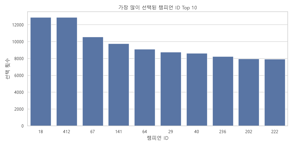
실제 챔피언명까지 알고 싶다면 별도의 챔피언 ID-이름 매핑 데이터가 필요하다.
import json

# 챔피언 ID-이름 정보 매핑
with open("dataset/champion_info_2.json", "r", encoding="utf-8") as f:
    champion_json = json.load(f)

champion_data = champion_json["data"]

id_to_name = {
    champ_info["id"]: champ_info["name"]
    for champ_info in champion_data.values()
}

t1_champ_cols = [
    "t1_champ1id",
    "t1_champ2id",
    "t1_champ3id",
    "t1_champ4id",
    "t1_champ5id"
]
t2_champ_cols = [
    "t2_champ1id",
    "t2_champ2id",
    "t2_champ3id",
    "t2_champ4id",
    "t2_champ5id"
]
champ_cols = t1_champ_cols + t2_champ_cols
for col in champ_cols:
    new_col = col.replace("id", "name")
    df[new_col] = df[col].map(id_to_name).fillna("Unknown")

ban_cols = [
    "t1_ban1", "t1_ban2", "t1_ban3", "t1_ban4", "t1_ban5",
    "t2_ban1", "t2_ban2", "t2_ban3", "t2_ban4", "t2_ban5"
]

for col in ban_cols:
    new_col = col + "_name"
    df[new_col] = df[col].map(id_to_name).fillna("Unknown")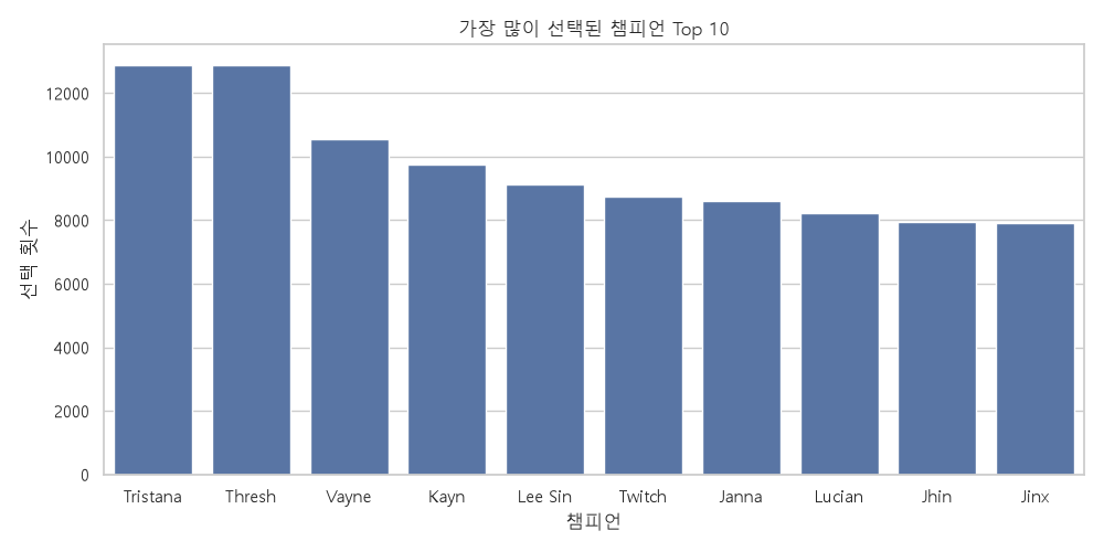
10. 데이터 누수(Data Leakage) 주의
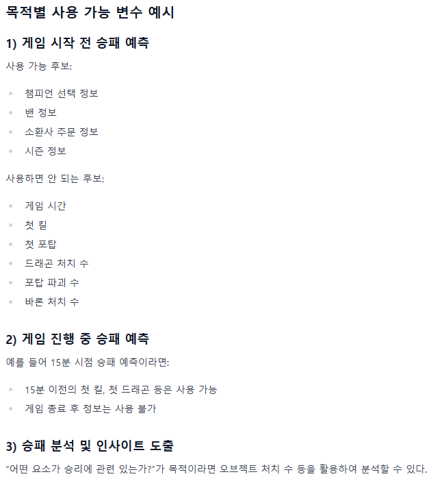
데이터 누수란 모델이 예측 시점에서 알 수 없는 미래 정보를 학습에 사용하는 문제다. 예를 들어 "게임 시작 전에 승패를 예측"하려고 한다면 다음 변수들은 사용할 수 없다.
post_game_cols = [
    "gameDuration",
    "t1_towerKills", "t2_towerKills",
    "t1_inhibitorKills", "t2_inhibitorKills",
    "t1_baronKills", "t2_baronKills",
    "t1_dragonKills", "t2_dragonKills",
    "t1_riftHeraldKills", "t2_riftHeraldKills"
]
15. 학습용 데이터 만들기
- 승리 팀을 0/1로 변경: 머신러닝에서는 보통 이진 분류 타겟을
0,1로 많이 사용한다.
# 승리 팀을 0과 1로 변경
df["target"] = (df["winner"] == 1).astype(int)
print(df[["winner", "target"]].head())
'''
   winner  target
0       1       1
1       1       1
2       1       1
3       1       1
4       1       1
'''- 게임 시작 전 예측용 데이터 구성 예시
# 게임 시작 전 예측용 데이터 구성
pregame_features = [
    "seasonId",

    "t1_champ1id", "t1_champ2id", "t1_champ3id",
    "t1_champ4id", "t1_champ5id",

    "t2_champ1id", "t2_champ2id", "t2_champ3id",
    "t2_champ4id", "t2_champ5id",

    "t1_champ1_sum1", "t1_champ1_sum2",
    "t1_champ2_sum1", "t1_champ2_sum2",
    "t1_champ3_sum1", "t1_champ3_sum2",
    "t1_champ4_sum1", "t1_champ4_sum2",
    "t1_champ5_sum1", "t1_champ5_sum2",

    "t2_champ1_sum1", "t2_champ1_sum2",
    "t2_champ2_sum1", "t2_champ2_sum2",
    "t2_champ3_sum1", "t2_champ3_sum2",
    "t2_champ4_sum1", "t2_champ4_sum2",
    "t2_champ5_sum1", "t2_champ5_sum2",

    "t1_ban1", "t1_ban2", "t1_ban3", "t1_ban4", "t1_ban5",
    "t2_ban1", "t2_ban2", "t2_ban3", "t2_ban4", "t2_ban5"
]

X = df[pregame_features] # 입력 데이터(특성, feature)
y = df["target"] # 맞히고 싶은 정답(타깃, target)
전처리 전체 코드 예시
import numpy as np
import pandas as pd
import matplotlib.pyplot as plt
import seaborn as sns

# 1. 데이터 불러오기
df = pd.read_csv("dataset/games.csv")

# 2. 기본 확인
print("데이터 크기:", df.shape)
print("\n결측치 개수:")
print(df.isnull().sum().sort_values(ascending=False).head(10))

print("\n중복 gameId 개수:")
print(df["gameId"].duplicated().sum())

# 3. 중복 제거
df = df.drop_duplicates(subset="gameId")

# 4. 시간 변환
df["creationTime"] = pd.to_datetime(
    df["creationTime"],
    unit="ms"
)

# 5. 경기 시간: 초 -> 분
df["gameDuration_min"] = df["gameDuration"] / 60

# 6. 타깃 생성
# 팀1 승리면 1, 팀2 승리면 0
df["target"] = (df["winner"] == 1).astype(int)

# 7. 팀 간 오브젝트 차이 변수 생성
df["tower_diff"] = df["t1_towerKills"] - df["t2_towerKills"]
df["inhibitor_diff"] = df["t1_inhibitorKills"] - df["t2_inhibitorKills"]
df["baron_diff"] = df["t1_baronKills"] - df["t2_baronKills"]
df["dragon_diff"] = df["t1_dragonKills"] - df["t2_dragonKills"]
df["riftHerald_diff"] = (
    df["t1_riftHeraldKills"] - df["t2_riftHeraldKills"]
)

# 8. 확인
print(df[[
    "winner",
    "target",
    "gameDuration_min",
    "tower_diff",
    "dragon_diff"
]].head())

# ---결과---
데이터 크기: (51490, 61)

결측치 개수:
gameId            0
creationTime      0
gameDuration      0
seasonId          0
winner            0
firstBlood        0
firstTower        0
firstInhibitor    0
firstBaron        0
firstDragon       0
dtype: int64

중복 gameId 개수:
437
   winner  target  gameDuration_min  tower_diff  dragon_diff
0       1       1         32.483333           6            2
1       1       1         30.850000           8            2
2       1       1         24.883333           6            0
3       1       1         29.300000           9            2
4       1       1         34.900000           6            2
EDA 및 전처리 순서 정리
- 데이터 불러오기
head(),shape,info(),describe()등으로 구조 확인- 결측치 확인
- 중복 데이터 확인
- 타깃 변수 분포 확인
- 주요 수치형 변수 분포 시각화
- 타깃와 주요 변수의 관계 분석
- 날짜/시간 데이터 변환
- 필요하면 차이 변수 생성
- 데이터 누수 변수 제거
- X(입력값), y(정답값) 생성
- 이후 머신러닝 모델 학습
'CS > Python' 카테고리의 다른 글
| 파이썬으로 모델 검증/해석 찍먹하기 (0) | 2026.08.07 |
|---|---|
| 파이썬으로 머신러닝 찍먹하기 (0) | 2026.08.07 |
| 파이썬으로 데이터 시각화 찍먹하기 (0) | 2026.08.06 |
| 파이썬의 Pandas 라이브러리에 대해 알아보기 (0) | 2026.08.06 |
| 파이썬의 NumPy 라이브러리에 대해 알아보기 (0) | 2026.08.05 |